THERMODYNAMICS & CYCLE ANALYSIS

Every state.
The whole cycle.

Build and refine cycle models in an engineering equation editor. Connect fluid properties, solved states, and process paths, then follow a design change through to performance.

Explore the workflow Get started

Rankine cycle state points and process paths on a temperature–entropy diagram — The Rankine cycle, traced through its state points.View full size

01 / CONNECT THE STATES

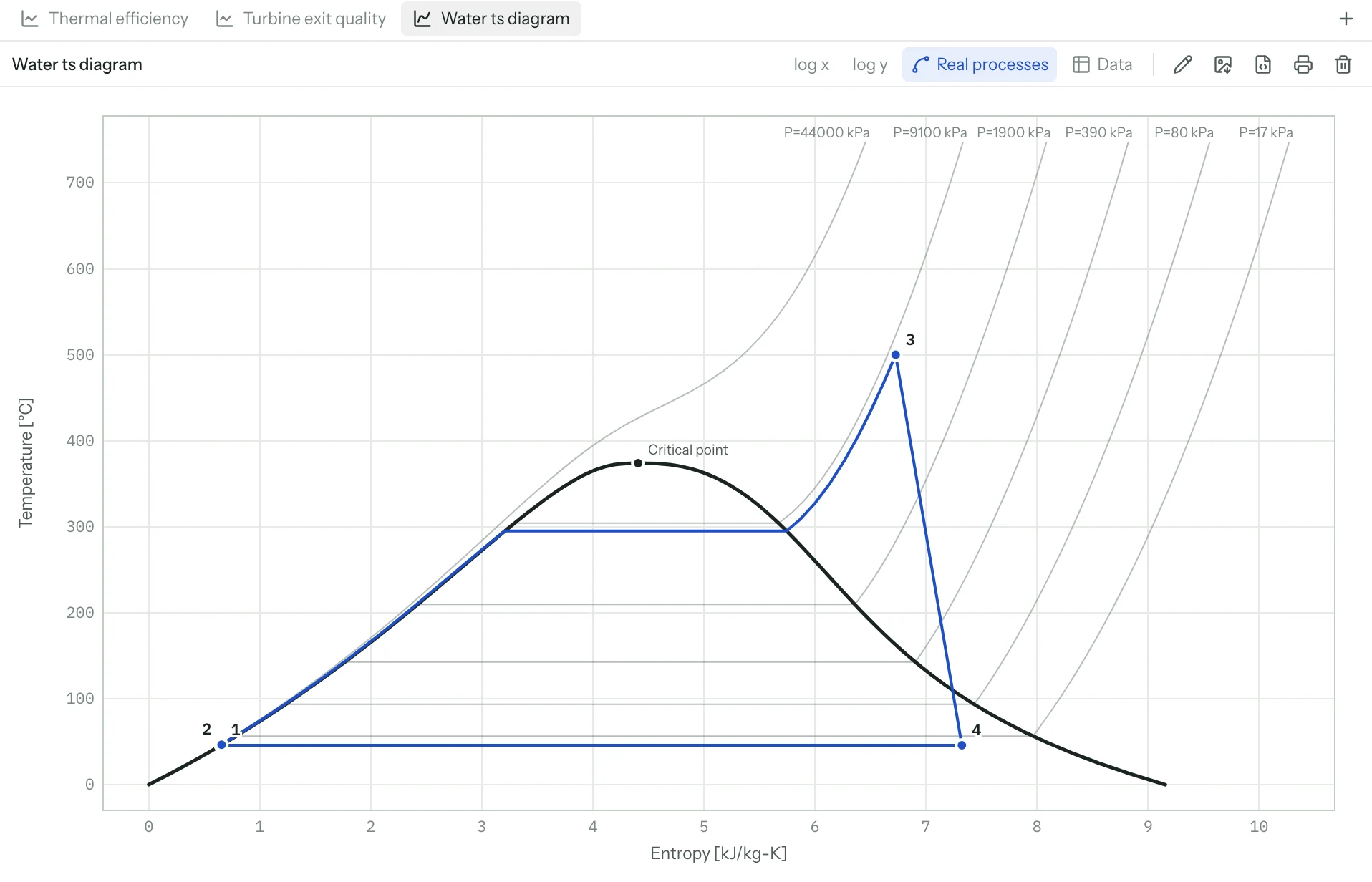
Follow each state through the system.

Build the cycle with the agent, then inspect the solved states. Change a pressure, temperature, or efficiency and follow its effect through the table and property diagram.

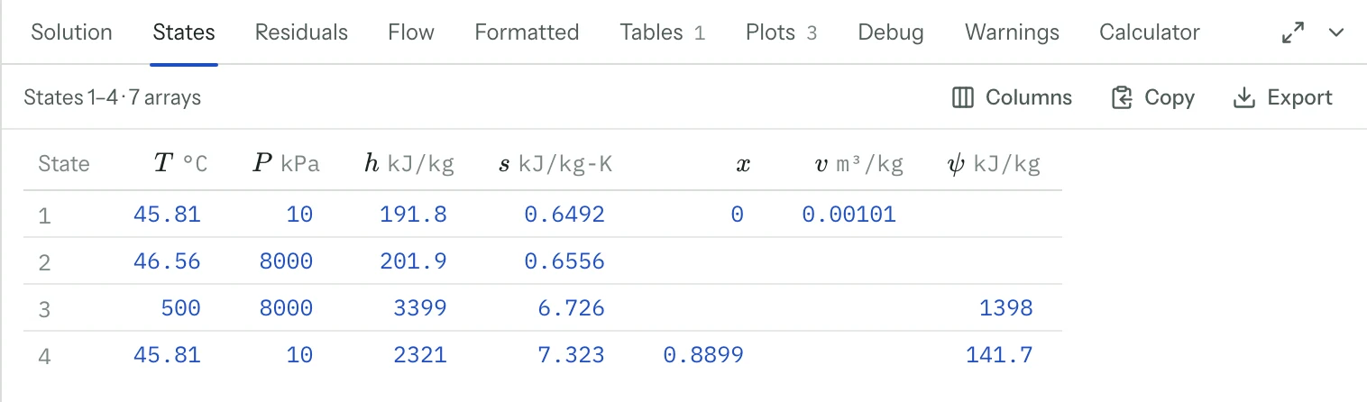
Rankine cycle States table with temperature, pressure, enthalpy, entropy, quality, specific volume and exergy — Arrays become state points. Select a value in the States table to return to its variable in the equations.View full size

Properties belong in the model.

Inspect enthalpy, entropy, density, and transport properties at each state. Autocomplete adapts the available property inputs to the selected fluid. The property-call builder lets you evaluate a call before inserting it into the model.

Process paths tell the story.

T–s, P–h, P–v, T–v, h–s, and psychrometric diagrams connect solved states. Recognized constant-property processes follow their paths through the diagram.

02 / COMPARE THE DESIGNS

Which input
moves the result?

Pin net power and efficiency, then drag a pressure input to see how both respond. Quick sweep plots the response across a range without setting up a table. A sensitivity chart helps you decide which inputs deserve a closer study.

Use Min/Max to search within bounds, and uncertainty propagation to see how input uncertainty reaches an output. Keep energy-balance checks visible with model assertions.

Plan a design comparison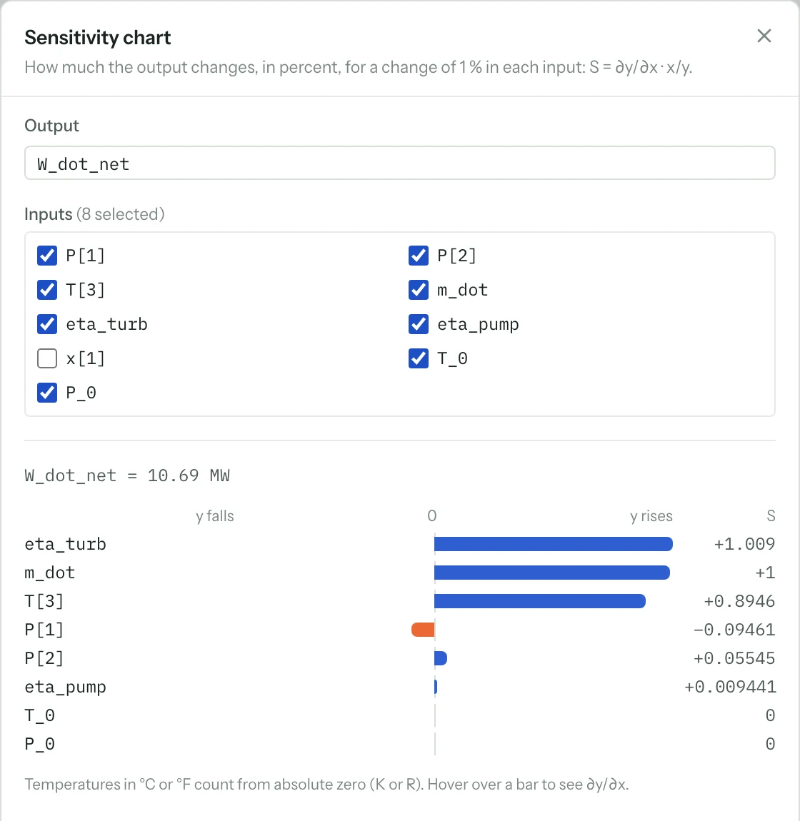

Rankine cycle sensitivity chart ranking the effect of inputs on net power — In this Rankine example, turbine efficiency and mass flow have the largest normalized sensitivities for net power.View full size

03 / SHARE THE REASONING

Make the result easy to review.

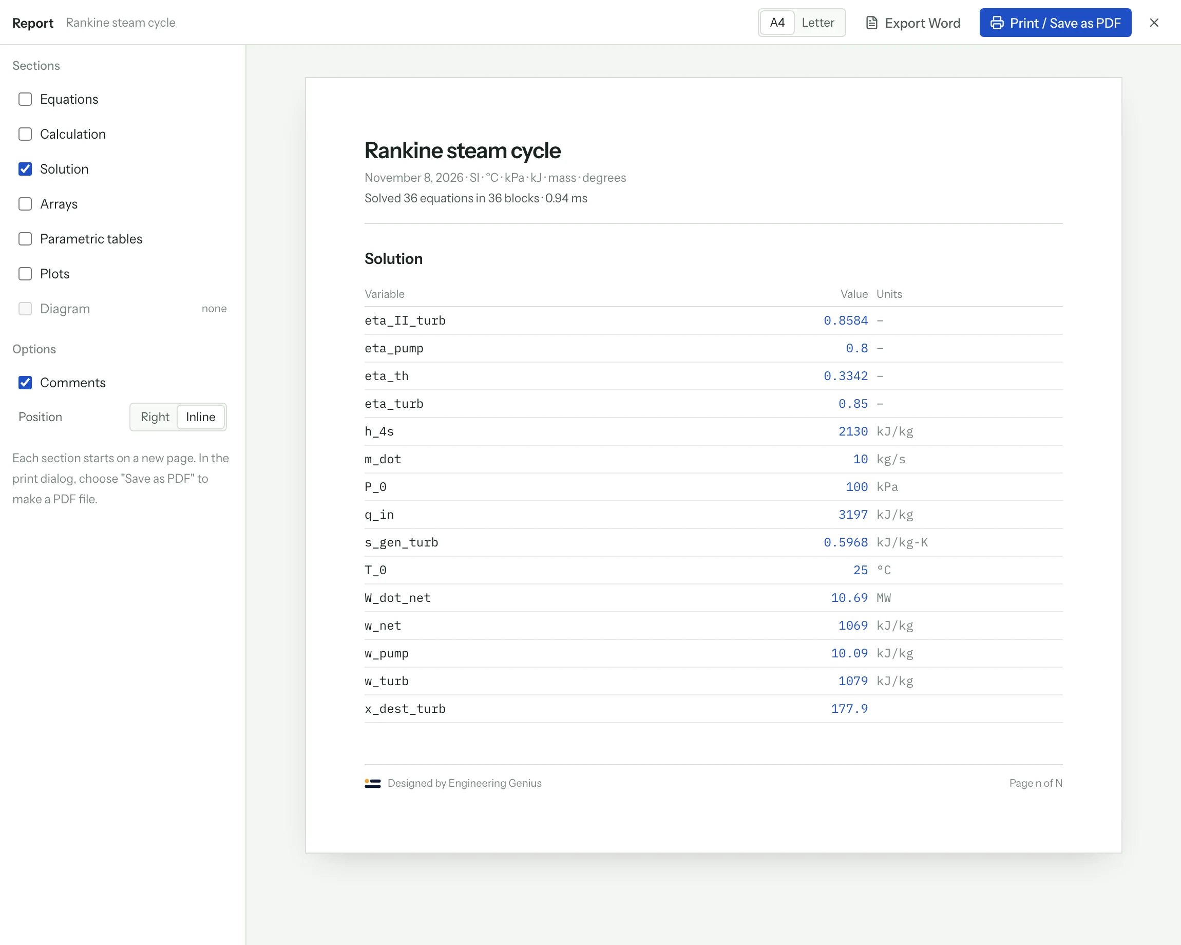
Carry the equations, substituted values, state tables, and plots into a calculation report. Or put inputs and outputs on a diagram and publish a calculation app.

Report builder showing the complete Rankine solution table, section choices, and Word and PDF export — Choose the sections your reviewer needs. Export Word, or use the browser’s print dialog to save a PDF.View full size

FROM A SOLVE TO A HANDOFF

The calculation
travels with
the conclusion.

Formatted calculations show the symbolic relationship, the values and units substituted into it, and the result.

A published calculation app gives colleagues a way to change inputs and solve in a browser.

Explore reports and sharing

CHOOSE A STARTING POINT

Different cycles.
The same connected workflow.

Steam power

Rankine cycle, water properties, component efficiencies, boiler-pressure study.

Refrigeration

Vapor-compression model, refrigerant properties, and P–h process paths.

Gas turbines

Air-standard Brayton cycle with compressor and turbine efficiencies.

Moist air

Cooling and dehumidification, condensate, and cooling load.

Built-in examples open as editable copies. Property coverage includes real fluids, refrigerant blends, ideal gases, moist air, and brines; review the ranges and reference states for your model.

FROM A QUESTION TO A WORKING MODEL

Build a cycle you can explain.

Describe the problem, review the model, and explore the alternatives.

Start with your problem Try the interactive examples